Bispectrum Module
The bispectrum module (bk) computes contributions to the galaxy bispectrum in redshift space, including wide-separation and relativistic corrections.
The bispectrum output is available as multipole moments or the full angle-dependent local bispectrum.
Bispectrum Multipoles
The bispectrum can be expanded in terms of the “Scoccimarro” spherical harmonic multipoles, which are defined with respect to the orientation of the triangle to the line-of-sight.
Here’s an example class from the bispectrum module:
- class bk.NPP
This class computes the Newtonian plane-parallel constant redshift terms.
Methods
- lx(cosmo_functions, k1, k2, k3=None, theta=None, zz=0, r=0, s=0, sigma=None)
Compute the x-th multipole ( l_x ) of the bispectrum for the Newtonian contribution.
- Parameters:
cosmo_functions (object) – An instance of ClassWAP containing cosmology and survey biases.
k1 (array-like) – Wavevector magnitude 1, broadcastable array in units of [Mpc/h].
k2 (array-like) – Wavevector magnitude 2, broadcastable array in units of [Mpc/h].
k3 (array-like) – (Optional) Wavevector magnitude 3, broadcastable array in units of [Mpc/h]. Either k3 or theta must be set.
theta (array-like) – (Optional) Outside angle θ, broadcastable array. Either theta or k3 must be set.
zz (array-like) – Redshift, broadcastable array with k vectors. Default is 0.
r (float) – Parameter r that sets the Line of Sight (LoS) in the local triplet. Default is 0.
s (float) – Parameter s that sets the Line of Sight (LoS) in the local triplet. Default is 0.
sigma (float) – (Optional) Linear dispersion that sets FoG damping. Default is None.
- Returns:
Bispectrum multipole contribution in units of [h/Mpc]^6.
- ylm(l, m, cosmo_functions, k1, k2, k3=None, theta=None, zz=0, r=0, s=0, sigma=None)
Compute the multipole (ell,m) of the bispectrum by performing the angular integral numerically.
- Parameters:
l (int) – The degree of the spherical harmonic.
m (int) – The order of the spherical harmonic.
cosmo_functions (object) – An instance of ClassWAP containing cosmology and survey biases.
k1 (array-like) – Wavevector magnitude 1, broadcastable array in units of [Mpc/h].
k2 (array-like) – Wavevector magnitude 2, broadcastable array in units of [Mpc/h].
k3 (array-like) – (Optional) Wavevector magnitude 3, broadcastable array in units of [Mpc/h]. Either k3 or theta must be set.
theta (array-like) – (Optional) Outside angle θ, broadcastable array. Either theta or k3 must be set.
zz (array-like) – Redshift, broadcastable array with k vectors. Default is 0.
r (float) – Parameter r that sets the Line of Sight (LoS) in the local triplet. Default is 0.
s (float) – Parameter s that sets the Line of Sight (LoS) in the local triplet. Default is 0.
sigma (float) – (Optional) Linear dispersion that sets FoG damping. Default is None.
- Returns:
Bispectrum multipole contribution in units of [h/Mpc]^6.
Available Bispectrum Classes
CosmoWAP provides multiple classes for different contributions to the bispectrum:
NPP: Newtonian plane-parallel (Kaiser)
WA1: First-order wide-angle corrections
WA2: Second-order wide-angle corrections
RR1: First-order radial-redshift corrections
RR2: Second-order radial-redshift corrections
WS: Full combined wide-separation terms (wide-angle + radial-redshift)
GR1: First-order relativistic corrections (H/k)
GR2: Second-order relativistic corrections (H/k)
Loc, Eq, Orth: PNG contributions (local, equilateral, orthogonal)
Note
PNG contributions (Loc, Eq, Orth) require compute_bias=True when initialising ClassWAP.
Each class follows the same interface with lx() methods for computing multipoles of order x, and a ylm() method for numerical integration of arbitrary multipoles.
LOS parameters (r, s): The line-of-sight direction d for the local triplet is defined as:
where r, s ∈ [0,1] and x_i are the triplet positions. Default r=s=0 corresponds to the “midpoint” LOS.
Full Local Bispectrum
In addition to the multipole decomposition, CosmoWAP also provides functions to compute the full angle-dependent local bispectrum.
- bk.Bk_0(mu, phi, cosmo_functions, k1, k2, k3=None, theta=None, zz=0, r=0, s=0, sigma=None)
Compute the angle-dependent Newtonian bispectrum.
- Parameters:
mu (float) – Cosine of the angle between the LOS and (k_1)
phi (float) – Azimuthal angle between LOS and (k_2) in plane normal to (k_1).
cosmo_functions (object) – An instance of ClassWAP containing cosmology and survey biases.
k1 (array-like) – Wavevector magnitude 1, broadcastable array in units of [Mpc/h].
k2 (array-like) – Wavevector magnitude 2, broadcastable array in units of [Mpc/h].
k3 (array-like) – (Optional) Wavevector magnitude 3, broadcastable array in units of [Mpc/h]. Either k3 or theta must be set.
theta (array-like) – (Optional) Outside angle θ, broadcastable array. Either theta or k3 must be set.
zz (array-like) – Redshift, broadcastable array with k vectors. Default is 0.
r (float) – Parameter r that sets the Line of Sight (LoS) in the local triplet. Default is 0.
s (float) – Parameter s that sets the Line of Sight (LoS) in the local triplet. Default is 0.
sigma (float) – (Optional) Linear dispersion that sets FoG damping. Default is None.
- Returns:
The bispectrum contribution, in units of [h/Mpc]^6.
The full angle-dependent bispectrum is available for the Newtonian contribution. For other contributions, use the multipole decomposition via the class methods.
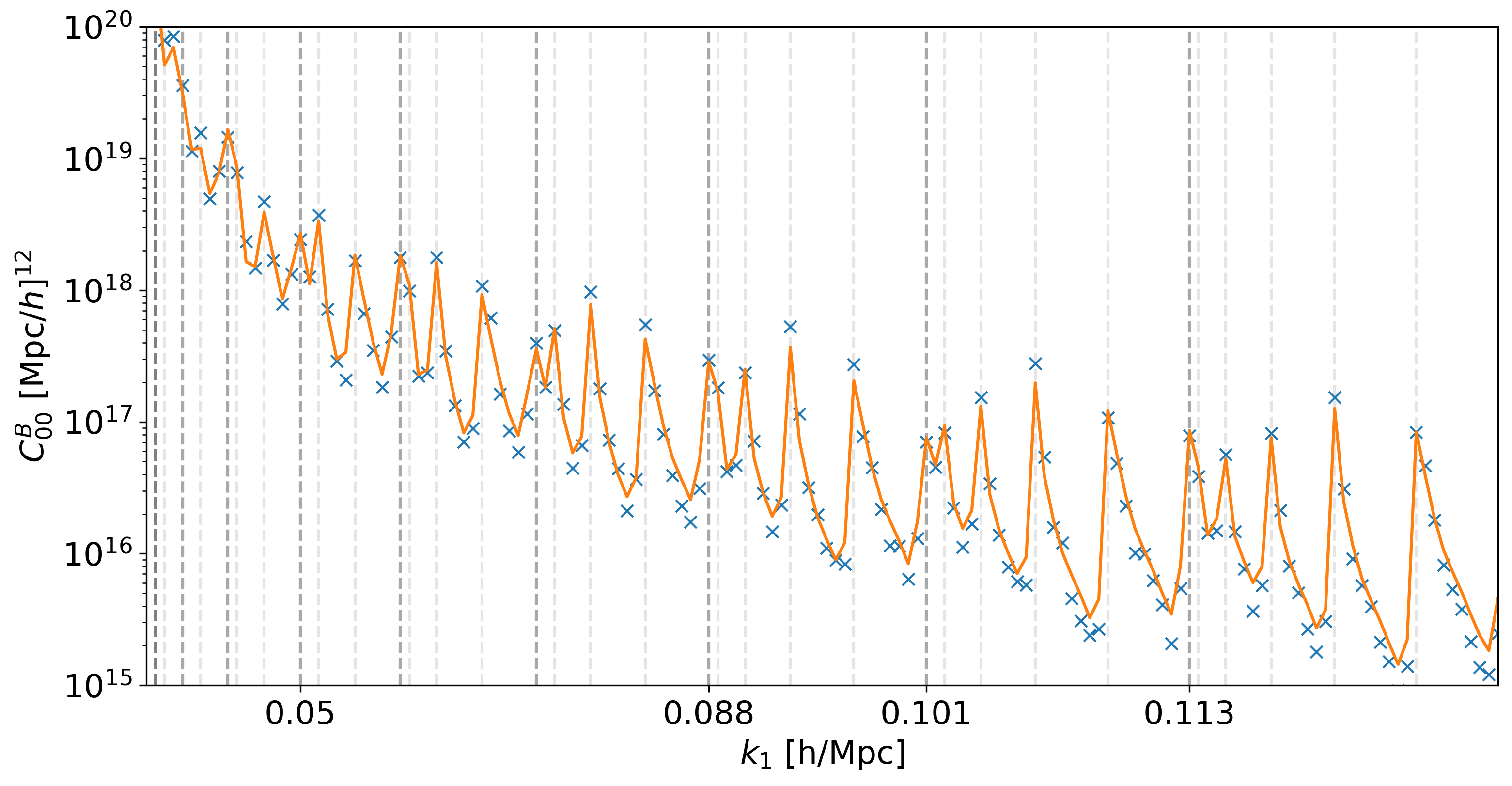
Bispectrum Gaussian Covariance
CosmoWAP also provides functionality to compute the Gaussian covariance of the bispectrum multipoles.
- class bk.COV(cosmo_functions, k1, k2, k3, theta, zz, r=0, s=0)
Compute the Gaussian covariance for bispectrum multipoles.
- Parameters:
cosmo_functions (object) – An instance of ClassWAP.
k1 (array-like) – First wavevector magnitude.
k2 (array-like) – Second wavevector magnitude.
k3 (array-like) – Third wavevector magnitude.
theta (array-like) – Outside angle of the triangle.
zz (float) – Redshift.
r (float) – Parameter r for LOS specification.
s (float) – Parameter s for LOS specification.
Methods
- Nab_cd()
Compute the covariance between ℓ1=a, m1=b and ℓ2=c, m2=d multipoles.
The notation is Nab_cd where a, b, c, d are the multipole and m-indices. For example, N00_00 is the covariance of the monopole (ℓ=0, m=0) with itself.
- Returns:
Covariance value.
Comparison with Sims
Gaussian covariance compared to the measured covariance from 100 fiducial Quijote Quijote sims.