Gaussian Covariance

CosmoWAP computes the Gaussian covariance of (multi-tracer) power spectrum and bispectrum multipoles, which are used in the forecasting modules.

The covariance pipeline uses the numerical \(\mu\) integration framework: the full \(P(k,\mu)\) is constructed from the pk_int kernel machinery (via pk.get_mu) for each term, then projected onto multipole covariances via Gauss-Legendre quadrature. This means that any combination of terms (Newtonian, wide-separation, relativistic, integrated effects) is handled through the same interface – this is particularly important for inclduing integrated contributions where there is a big speedip.

Power Spectrum Covariance

For full details see Appendix B of 2511.090466. But briefly…

The Gaussian covariance of the power spectrum multipoles is:

\[C[P^{ab}_{\ell_1}, P^{cd}_{\ell_2}](k) = \frac{(2\ell_1+1)(2\ell_2+1)}{N_k} \int \frac{d\Omega_k}{4\pi}\, \mathcal{L}_{\ell_1}(\mu) \left[ \mathcal{L}_{\ell_2}(\mu)\, \tilde{P}^{ac}(k,\mu)\, \tilde{P}^{bd*}(k,\mu) + \mathcal{L}_{\ell_2}(-\mu)\, \tilde{P}^{ad}(k,\mu)\, \tilde{P}^{bc*}(k,\mu) \right]\]

where \(\hat{P}^{ab}(\bm{k},\bm{d}) = P^{ab}_{\rm loc}(\bm{k},\bm{d}) + \frac{\delta^K_{a,b}}{n_a}.\) includes shot noise and the indices \(a,b,c,d\) label tracer populations.

Each \(P(k,\mu)\) is built by pk.get_mu, which uses the pk_int kernel machinery to evaluate the full angle-dependent power spectrum for a given term (e.g. 'NPP', 'GR2', 'IntNPP'). The \(\mu\) integral is then performed via Gauss-Legendre quadrature with n_mu nodes.

Bispectrum Covariance

For full details see Section 4.1.1 of Addis (2026) Constraints and biases: Joint power spectrum and bispectrum forecasts on ultra-large scales.

The Gaussian covariance of the bispectrum spherical harmonic multipoles is for single-tracer - see Addis (2026) for the full multi-tracer expression:

\[C[B_{\ell_1 m_1}, B_{\ell_2 m_2}](k_1, k_2, k_3) = \frac{1}{N_{\rm tri}} \int \frac{d\Omega_k}{4\pi}\, 4\pi\, Y^*_{\ell_1 m_1}(\hat{k})\, Y_{\ell_2 m_2}(\hat{k}) \, \tilde{P}(k_1,\mu_1)\, \tilde{P}(k_2,\mu_2)\, \tilde{P}(k_3,\mu_3)\]

where \(\mu_i = \hat{k} \cdot \hat{k}_i\) and the integration is over the orientation of the triangle relative to the line of sight.

The same pk.get_mu is used to build each of the three \(P(k_i, \mu_i)\), and the integration is now 2D over \((\mu, \phi)\) using Gauss-Legendre quadrature with n_mu and n_phi nodes respectively. The spherical harmonics \(Y_{\ell m}\) replace the Legendre polynomials used in the power spectrum case. FoG damping is applied independently to each triangle leg via \(e^{-(k_i \mu_i)^2 \sigma^2 / 2}\).

Multi-Tracer Covariance

For Fisher forecasting, the full multi-tracer multipole covariance is needed. This is handled by FullCovPk and FullCovBk in the forecast module, which are called internally by FullForecast.get_fish().

FullCovPk

class forecast.covariances.FullCovPk(fc, cf_mat, cov_terms, sigma=None, n_mu=64, fast=False, nonlin=False, kernels=True)

Multi-tracer power spectrum multipole covariance for a single redshift bin.

Parameters:

fc – PkForecast instance
cf_mat (list) – List of ClassWAP instances for each tracer combination
cov_terms (list) – Terms to include (e.g. ['NPP', 'GR2', 'IntNPP'])
sigma (float) – FoG damping
n_mu (int) – Number of Gauss-Legendre nodes for \(\mu\) integration (default: 64)
fast (bool) – Use symmetry to integrate over \([0,1]\) only
nonlin (bool) – Use HALOFIT power spectra in covariance
kernels (bool) – Work directly with pk_int kernels (default). If False, use \(P(k, \mu)\) expressions directly.

get_cov(ln, sigma=None)

Compute the full covariance matrix for the given list of multipoles.

Parameters:: ln (list) – Multipole orders (e.g. [0, 2, 4])
Returns:: Array of shape (N_data, N_data, N_k)

For single-tracer, the data vector is \(\{P_{\ell_1}(k), P_{\ell_2}(k), \ldots\}\) and the covariance has shape (len(ln), len(ln), N_k).

For multi-tracer (bright/faint split), even multipoles have three tracer spectra (\(P^{BB}_\ell, P^{BF}_\ell, P^{FF}_\ell\)) while odd multipoles have only the cross-spectrum (\(P^{BF}_\ell\)). The covariance matrix accounts for all cross-correlations between tracer combinations and multipoles.

FullCovBk

class forecast.covariances.FullCovBk(fc, cf_mat, cov_terms, sigma=None, n_mu=64, n_phi=32, fast=False, nonlin=False, kernels=True)

Multi-tracer bispectrum multipole covariance for a single redshift bin.

Parameters:

fc – BkForecast instance
cf_mat (list) – List of ClassWAP instances for each tracer combination
cov_terms (list) – Terms to include
sigma (float) – FoG damping
n_mu (int) – Gauss-Legendre nodes for \(\mu\) (default: 64)
n_phi (int) – Gauss-Legendre nodes for \(\phi\) (default: 32)
fast (bool) – Use symmetry to halve the \(\mu\) range
nonlin (bool) – Use HALOFIT power spectra
kernels (bool) – Work directly with kernels (default). If False, use Bk expressions directly.

get_cov(ln)

Compute the full covariance matrix.

Parameters:: ln (list) – Multipole orders (e.g. [0])
Returns:: Array of shape (N_data, N_data, N_tri)

For multi-tracer bispectrum, the tracer combinations are \(B^{BBB}, B^{BBF}, B^{BFF}, B^{FFF}\), giving a (4*len(ln), 4*len(ln), N_tri) covariance matrix.

Caching

Both FullCovPk and FullCovBk precompute and cache \(P(k,\mu)\) for all terms and tracer combinations during initialisation (create_cache). The \(\mu\) integration for different multipole pairs then reuses these cached values, avoiding redundant evaluations of the power spectrum – this is the most expensive step, particularly when integrated effects are included.

Nonlinear Corrections

Nonlinear corrections to the covariance can be included in two ways:

``nonlin=True`` in ``FullCovPk``/``FullCovBk``: Replaces the linear \(P(k)\) with the HALOFIT nonlinear power spectrum throughout the covariance.
``nonlin=True`` in ``bk.COV.cov()``: Adds nonlinear correction following Eq. 27 of 1610.06585, replacing the linear \(P(k_i)\) with \(\Delta P(k_i) = P^{\rm NL}(k_i) - P^{\rm lin}(k_i)\) for each triangle leg in turn.

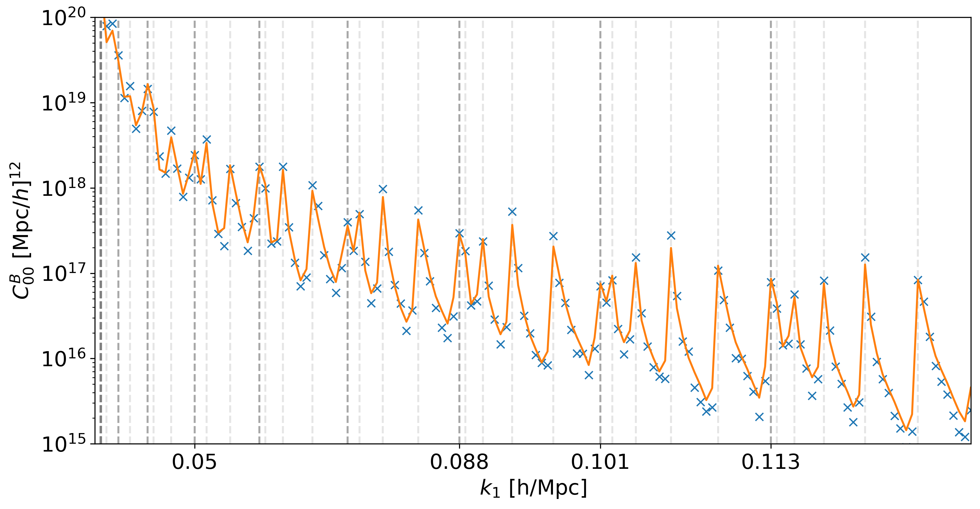
Comparison with Simulations

Gaussian covariance compared to the measured covariance from 100 fiducial Quijote simulations.

Comparison of theory to measured covariance

Analytical Expressions

Analytically-mu multipole covariance expressions (exported from Mathematica) are also available for the Newtonian tree-level case, optionally including FoG damping.

Power spectrum: pk.COV provides methods N00(), N20(), N22(), N40(), N42(), N44() (even) and N11(), N31(), N33() (odd) for \(C[P_{\ell_1}, P_{\ell_2}](k)\).
Power spectrum numerical: pk.COV_MU provides cov_l1l2(term1, term2, l1, l2, ...) for numerically integrating arbitrary term pairs.
Bispectrum: bk.COV provides analytical multipole methods (e.g. N00(), N20(), N00_00()) with naming convention Nab_cd for \(C[B_{\ell_1=a,m_1=b}, B_{\ell_2=c,m_2=d}]\). When sigma is set, bk.COV automatically switches to numerical \(\mu\)-\(\phi\) integration via its ylm() method.